
Full-Stack / TypeScript
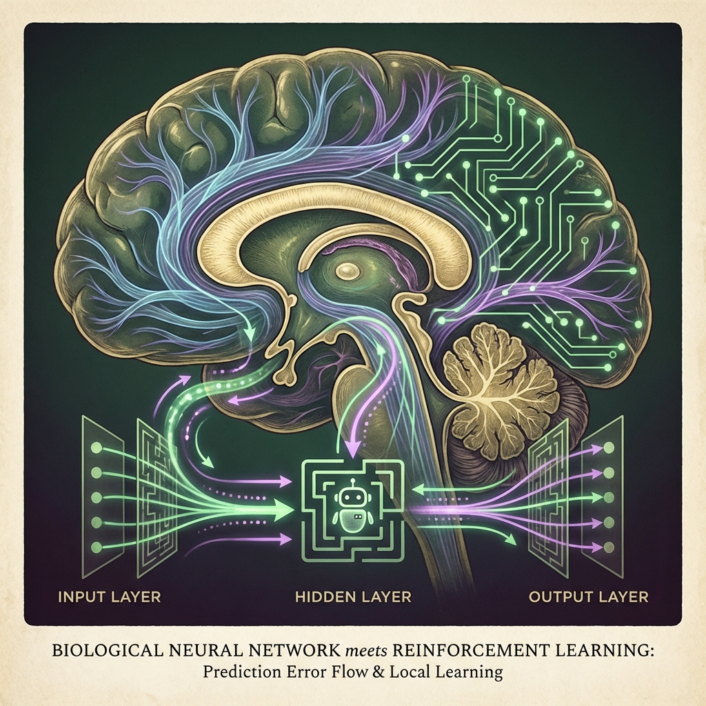
Reinforcement learning using Predictive Coding principles, where intelligent behavior emerges from local prediction errors rather than backpropagation.
Traditional reinforcement learning relies on backpropagation—gradients flowing backward through time and across network layers. But biological brains don’t have a “backward pass.” Neurons learn locally based on their immediate inputs and outputs.
PC-RL demonstrates that intelligent behavior can emerge from purely local learning rules, where each node simply tries to minimize its prediction error.
The simplified learning PC network shows clear advantages:
| Agent | Success Rate |
|---|---|
| Random PC | 35% |
| Learning PC | 100% |
Key achievements:
In predictive coding, each node in a hierarchy:
Learning is entirely local—no global loss function, no backward pass.
In PC-RL, we structure the network to learn action-outcome associations:
┌─────────────────────────────────────────────┐
│           Higher PC Layers                  │
│    (predict state transitions, rewards)     │
└─────────────────────────────────────────────┘
                    ▲
                    │ prediction errors
                    │
┌─────────────────────────────────────────────┐
│           Action Nodes                       │
│    (predict outcomes for each action)       │
│    ┌───────┐ ┌───────┐ ┌───────┐           │
│    │ Act 0 │ │ Act 1 │ │ Act 2 │ ...       │
│    └───────┘ └───────┘ └───────┘           │
└─────────────────────────────────────────────┘
                    ▲
                    │ state input
                    │
┌─────────────────────────────────────────────┐
│           Sensory Layer                      │
│         (environment state)                 │
└─────────────────────────────────────────────┘
Actions are selected based on which action node has the lowest prediction error for desired outcomes:
def select_action(self, state, goal):
    errors = []
    for action_node in self.action_nodes:
        # What does this action predict will happen?
        predicted_outcome = action_node.predict(state)
        # How far is that from our goal?
        error = self.compute_error(predicted_outcome, goal)
        errors.append(error)

    # Choose action with lowest error to goal
    # (with some exploration noise)
    return softmax_sample(-np.array(errors) / temperature)
After taking an action and observing the outcome:
def learn(self, state, action, outcome):
    action_node = self.action_nodes[action]

    # What did we predict?
    predicted = action_node.predict(state)

    # What actually happened?
    actual = outcome

    # Local update to reduce this error
    action_node.update(predicted, actual)
No gradients through time. No global optimization. Just local error minimization.
PCAgent/
├── src/
│   ├── pc_node.py              # Basic PC node with local learning
│   ├── action_node.py          # Action nodes for RL interface
│   ├── pc_network.py           # Hierarchical network
│   ├── temporal_pc_node.py     # Adds eligibility traces
│   ├── learning_pc_network.py  # Full temporal PC
│   └── simple_learning_pc.py   # Simplified but effective
├── environments/
│   ├── simple_control.py       # Position control, grid world
│   └── gymnasium_wrapper.py    # Standard RL benchmarks
├── visualizations/
│   └── pc_dynamics_viz.py      # Real-time visualization
└── demos/
    ├── demo.py                 # Basic demonstration
    ├── demo_learning.py        # Learning comparison
    └── visualize_demo.py       # PC dynamics
class PCNode:
    def __init__(self, input_dim, output_dim):
        self.weights = np.random.randn(output_dim, input_dim) * 0.1
        self.prediction = np.zeros(output_dim)
        self.error = np.zeros(output_dim)

    def predict(self, input):
        self.prediction = self.weights @ input
        return self.prediction

    def compute_error(self, target):
        self.error = target - self.prediction
        return self.error

    def update(self, learning_rate=0.01):
        # Local Hebbian-like update
        self.weights += learning_rate * np.outer(self.error, self.input)
For RL, we need to handle delayed rewards. The temporal PC node adds eligibility traces:
class TemporalPCNode(PCNode):
    def __init__(self, *args, trace_decay=0.9):
        super().__init__(*args)
        self.eligibility_trace = np.zeros_like(self.weights)
        self.trace_decay = trace_decay

    def update_trace(self, input):
        # Trace decays over time
        self.eligibility_trace *= self.trace_decay
        # Current activity adds to trace
        self.eligibility_trace += np.outer(self.prediction, input)

    def update_from_reward(self, reward):
        # Reward modulates trace for credit assignment
        self.weights += reward * self.eligibility_trace
PC-RL maintains several properties of biological learning:
| Property | Standard RL | PC-RL |
|---|---|---|
| Weight transport | Required (backprop) | ❌ Not needed |
| Global error signal | Required | ❌ Only local errors |
| Symmetric weights | Often assumed | ❌ No assumption |
| Continuous time | Discrete updates | ✅ Can be continuous |
| Local learning | ❌ Global optimization | ✅ Only local info |
Agent must move to a target position in 2D space:
env = PositionControlEnv(target=[0.5, 0.5])
agent = SimpleLearningPC(state_dim=2, action_dim=4)

for episode in range(100):
    state = env.reset()
    while not done:
        action = agent.select_action(state, goal=env.target)
        next_state, reward, done = env.step(action)
        agent.learn(state, action, next_state, reward)
        state = next_state
Discrete navigation with sparse rewards:
Intelligence doesn’t require global optimization. Local prediction error minimization, when structured correctly, can produce adaptive behavior indistinguishable from traditionally-trained RL agents—while being far more biologically realistic.


